Useful Tools

Building a One-Page Calendar

Kevin Pretorius Useful Tools 07 March 2023

A One-Page Calendar

Yesterday, I was inspired by a simple, but clever idea for a one-page calendar that I read about in Ethan Siegel's column in Big Think (see One Page Calendar)

It's not the sort of calendar that you write your dental appointment on, but it is great for answering questions like - which day of the week does my birthday fall on this year? or when do the clocks go forward in the UK (ie which is the last Sunday in March)?

What intrigued me, in particular, was whether an automated version of this could be built in Excel, just using Excel formulae and no VBA software. It turned out that it can, and it struck me as an excellent opportunity for a quick Excel tutorial, so here's how I did it, step by step.

How the Calendar Works

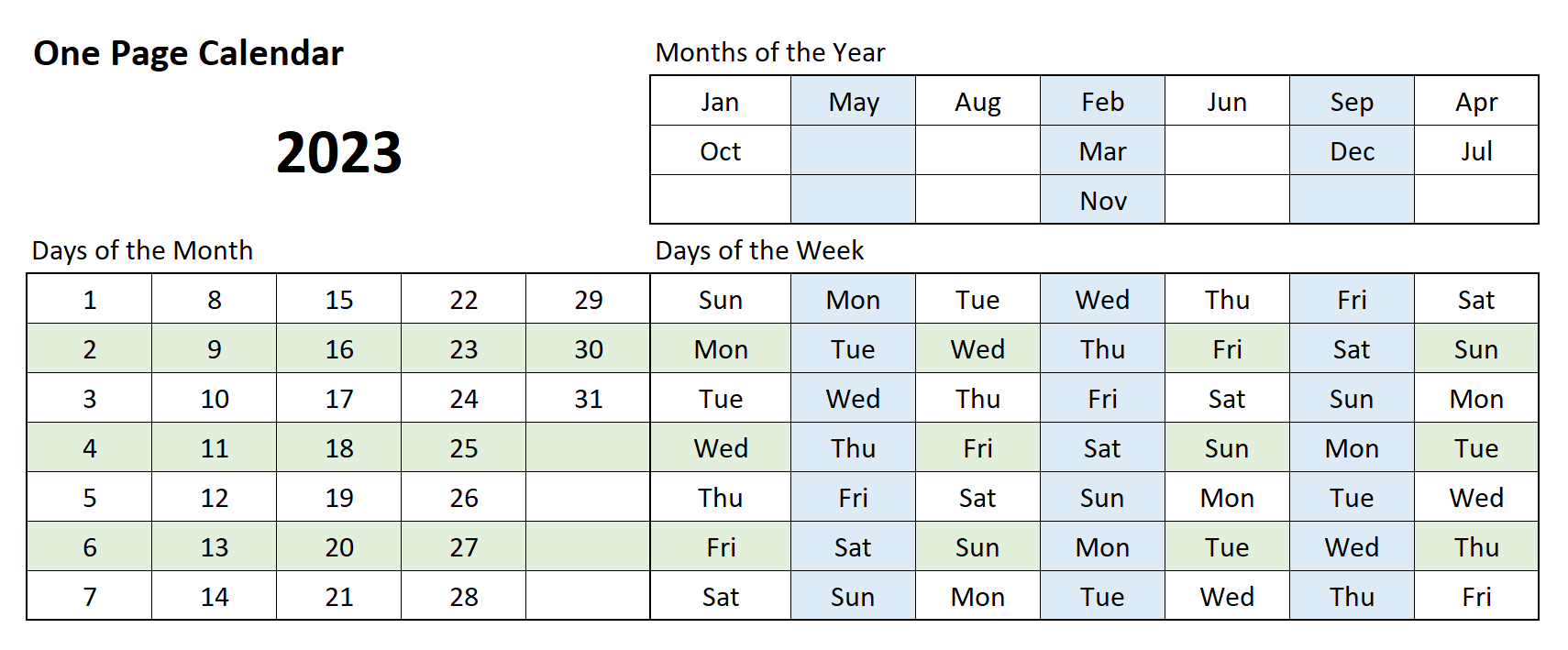
The one-page calendar is a simple table that ties together dates, months, and days of the week in a very easy-to-understand and intuitive fashion.

So let's say that you're planning a surprise for someone's birthday on Aug 6th and need to know what day of the week that is. Find the column for August, and the row for the 6th, and where they cross is a Sunday, so that's ideal for a day out.

Want to know the date of the 2nd Tuesday in February? Well, find the column with February, glance down the column to find Tuesday, and look across to see all the dates that fall on a Tuesday. The second entry is the 14th.

Planning a June wedding? Here are all the Saturdays...

If you're feeling adventurous, you might even try answering the question - which months have 5 Saturdays?

OK, I'm sure you get the idea. If you want more examples and information, please see Ethan's original article.

So why am I talking about this? It's because it's a fun and interesting question to think about how to build one of these with Excel, and particularly one that updates itself each year. Here's how I did that.

Days of the Month and Days of the Week

The Days of the Month and the Days of the Week tables don't change from year to year. If you wanted, you can just type them in (as numbers) and skip this section. But I'm going to use this opportunity to show how the SEQUENCE and WRAPCOLS functions can take care of this.

Let's start with the days of the month. Here I've used the SEQUENCE function to generate a list of numbers from 1 to 31, and then WRAPCOLS to present these as a series of columns, 7 cells high, padded with blanks when we run out of numbers. This formula is used just once, in cell B14.

Now you're probably more used to the idea of a formula returning a single value, but that isn't always true. In this case, the SEQUENCE function generates 31 values, and they spill over to adjacent cells.

SEQUENCE and WRAPCOLS are relatively recent functions, so if you're not yet using the latest version of Excel on a PC, these might not be available. But that's OK, you can simply type out these 31 values by hand. As you see, I've also added a little formatting, centered the numbers, coloured the background, and I've added some borders to make this look nicer.

The next step is to create the days of the week. For reasons that will become clear later, we'll represent these as the numbers 1 to 7.

Here I've used 7 SEQUENCE formulae in cells G14:G20 each generating 7 numbers along each row, starting from 1,2,3 etc. For convenience, I've used the value in column B as the starting value for each sequence.

To convert these all to the range 1..7 we need to use the MOD formula, as in...

=MOD(SEQUENCE(1,7,B14-1,1),7)+1

MOD(<number>,7) tells the function to only use the 7 numbers 0..6 and then wrap around when <number> is bigger than this. This is (a bit) like a clock only uses 12 numbers, making 13:00 the same as 1 o'clock for example. However we want 1..7 (not 0..6) when enumerating the days of the week, so we need to add 1 to whatever MOD returns, and start our sequences 1 value earlier to compensate.

Here's what that produces...

So how do you get this to display days of the week? By using custom number formatting.

First, select G14:M20 as the range of cells you want to format, go to the "Number Format" dropdown, and click on "More Number Formats..." at the bottom

In the dialog box, select Custom format, and type "ddd" (without the quotes) into the box, which tells Excel to format those numbers 1..7 as "Sun","Mon","Tue" etc. Click OK to apply this format.

And here's the result.

The Months of the Year

Everything we've built so far is static. It doesn't change from year to year. The more challenging part is the Months of the Year display, which changes every year, so we have to work out how to do that.

But let's first start with the year display. First I merged cells C10:E12, typed in =YEAR(TODAY()) to produce a display of the current year, applied a large 26pt, bold font size, and named this cell for easy future reference by typing "Current_Year" in the box as shown. Nice and easy.

So what's the secret of the Months of the Year display? Well (for example) May appears in the second column because the 1st of May occurs on Monday, the second day of the week. And Mar appears in the 2nd row of the 4th column, because it's the second month in the year that starts on a Wednesday. Performing this only using formulae is going to be a little complicated, so let's take this one step at a time.

First, we figure out which day of the week each month starts on. We can do this with a single formula written into cell B3. We use SEQUENCE(1,12) to generate the numbers 1..12, we turn this into twelve first-of-the-month dates for this year using DATE(<year>,<month>,1). Note that for <year> we reference the named cell Current_Year (or you could just write C10), <month> uses the sequence we generated, and 1 gives us the first of the month in each case. Finally, we use WEEKDAY to return the number of the day of the week those twelve first-of-the-month dates occur on.

So in the example, Jan 2023 begins on the 1st day of the week (Sun), Feb and March begin on the 4th day of the week (Wed) and so on.

And to make this look more readable, we format these numbers as days, which is what they represent of course. No change of formula, they're still just numbers 1..7, they just appear as days of the week now.

Now here's the most complicated bit. We're trying to figure out where the months need to be placed over the Days of the Week table.

So for example, above the Saturday entry (Cell M14) we want to know which months start on a Saturday. We could do this manually, by scanning across our "1st weekday" table, looking for Saturdays. We can see 2 examples: in the 4th column (ie April) and 7th column (ie July), and so we'd write 4 and 7 into that column of our table.

But how can we do that with a formula? Well, it can be done with the formula shown below.

=IFERROR(MATCH(G$14,OFFSET($B$3#,0,G4),0)+G4,"")

Here's how it works.

$B$3# means the spill range of values produced by the formula in B3, ie the range B3:M3

OFFSET(<range>,<rows>,<cols>) displaces a range by the specified number of rows and cols.

So OFFSET($B$3#,0,G4) means the range that's G4 places to the right of the range defined by $B$3#. At the moment G4 is blank (essentially 0), so has no effect.

MATCH(G$14,<range>) then looks in this range for the day of week we want, and returns how far along the first match is. So in cell G5, this formula looks along the range for a Sunday, and finds one in the first position, returning a 1.

So why use the OFFSET function? Well if we copy this formula in G5, down to the cell below (ie G6), we can repeat the search for months beginning with a Sunday, but we want to skip the one we just found. So by searching in a range shifted one cell to the right (ie C3:N3), we can avoid finding the first Sunday on the list. That's the point of OFFSET($B$3#,0,G5).

What MATCH then returns is the answer that the next Sunday is 9 months later than the first, so we then need to add the first month found (in this case January (month 1)) to get back that the second occurrence is in month 10 (October). This is why the result is MATCH(....)+G5.

And finally, if MATCH doesn't succeed, it throws up an error message, so we use IFERROR() to trap this, and substitute a blank. That's it!

Copy the formula to fill every cell in G5:M7, and you have a list of month numbers aligned over the correct starting days, which is always correct for the current year, and automatically updates itself.

The final step is simpler. We just want to convert these numbers to readable month names. There are several ways to do this, but this formula in G10...

=IF(ISNUMBER(G5),DATE(Current_Year,G5,1),"")

...tests to see if there's a number in the top table, and if so, creates a date out of it. And then (just as we did to display days as numbers) we use number formatting on the result, this time using a custom number format of "mmm".

And that's it. Here's the result.

You can hide rows 1..7 if you wish, and/or you can select the area you want to print (A8:N21) and use Print Layout / Print Area / Set Print Area, to ensure that only those cells appear on the print-out.

And we're done.

Sorting Photos with Excel

Kevin Pretorius Useful Tools 07 March 2023

I recently treated myself to a new laptop, and like any new computer owner, was working through the tedious process of migrating old files across from the previous computer. Now it seemed a great opportunity to do a little spring cleaning too, and so I thought it would be timely to clean up and sort through my old photos and to throw out any I really didn’t need anymore and were just taking up space.

As it happens, I dabble a little with astrophotography, where it’s commonplace to take hundreds of individual pictures and to combine them to produce a finished product, so I had shedloads of raw images I could potentially remove from my drive.

But as I searched through hundreds of folders, this quickly became a chore...

You literally have to click your way up and down the folder hierarchy, searching for where hundreds of junk photos might be, with little clue whether you’ve found them all, or where others might be hiding.

What I wanted was a map. Some kind of picture that showed me visually where the big folders and the big files were, without having to look for them myself.

Here’s what I came up with…

This image was generated on demand using VBA code running in Excel.

Here you can see my Pictures folder in red on the left, and subfolders of that in the next column, etc until (mostly towards the right) we see individual files shown. Each folder and file are drawn in proportion to their size, and the larger ones are labelled with their names and sizes too. Tiny files (less than a pixel tall) are not shown.

For a quick overview of how much storage is used and where – this is ideal.

Say for example, you were trying to move these files and only had a 10GB storage device to do it with. It's easy to see that you could probably move folders 2013 to 2016 in one batch, 2017 (at a pinch) in a second batch, and 2018 onwards for the rest.

But say 2017 was still too big, and you needed to check whether you could free up any files to make that really work. So this is why I added some clickable yellow arrows, which rebuild the folder map from a lower (or higher) starting point to make exploration a doddle.

In the image below, I’ve clicked the right-arrow on the 2017_08 USA Holiday to produce a more detailed picture of the folder hierarchy from that point downwards. I can see that I have lots and lots of photos were taken in Las Vegas (maybe I could afford to delete a few?) and I see a couple of large files (probably videos) of the Bellagio Fountains and our flight in a Helicopter. However there's one really big .mp4 file we shot in Yellowstone park, and doing something about that, might produce a more immediate win. Perhaps I could migrate that separately, (and therefore get the 2017 folder below that 10GB storage limit), or perhaps I could edit/trim the video to a smaller filesize, or even delete it completely (if the subject wasn't actually as interesting as it seemed at the time). What I choose to do with it doesn’t matter – the point is, that the information to tell you which folders and files need your attention - is all made highly visible.

To build this display in Excel, I wrote code in VBA to recursively descend down the file hierarchy from a user-selected start point – i.e. one selected with a folder browser. In each folder the code would iterate through each of the files, noting their name and size, and building a hierarchical data structure to represent the files and folders (using collections of collections) and propagating size totals up the hierarchy.

The display above can then be produced by ‘walking’ that hierarchy to produce the graphic you see. The graphics were drawn as 3D shaded rectangles onto a blank canvas provided by a Chart sheet. I added yellow arrows near the top right of every large rectangle, and assigned macros to rebuild the hierarchy from the indicated folder. To achieve this using just one callback, I check the identity of the calling shape in the callback code, and retrieve the full-path folder name which is written (invisibly) as a text label on each arrow.

The above coding is not excessively complex but produces a really useful display.